Statistics II - Extra Activity 5
Activity Overview
This activity uses a simulation study to illustrate the Central Limit Theorem (CLT). For this analysis, I utilized the california_housing dataset from the sklearn library, specifically focusing on the target variable (Median House Value).
What is the Central Limit Theorem?
The Central Limit Theorem states that for a population with any distribution shape, provided it has a finite mean ($\mu$) and finite standard deviation ($\sigma$), the distribution of sample means (or standardized sums) will approximately be a normal distribution as the sample size ($n$) increases.
We investigate two cases in this simulation:
- Case I (Sample Means): The distribution of sample means approaches a normal distribution with mean $\mu$ and standard deviation $\sigma/\sqrt{n}$.
- Case II (Sum of Sample Values): The standardized sum of the sample values approaches a standard normal distribution.
Colab for Simulation
1. Population Statistics
First, we load the data and calculate the population parameters.
import numpy as np
import pandas as pd
import seaborn as sns
import matplotlib.pyplot as plt
from sklearn.datasets import fetch_california_housing

# Set style
sns.set_style("whitegrid")

# 1. Load California Housing dataset
data = fetch_california_housing()
population_data = data.target

# 2. Calculate Population Statistics
pop_mean = np.mean(population_data)
pop_std = np.std(population_data)

print(f"--- Population Statistics ---")
print(f"Size of Data: {len(population_data)}")
print(f"Population Mean (μ): {pop_mean:.4f}")
print(f"Population Std Dev (σ): {pop_std:.4f}")
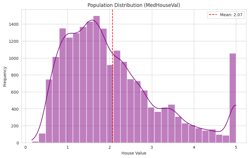
Based on the convergence of the “Mean of Means” in the results below, the Population Mean ($\mu$) is approximately 2.069, and the Population Standard Deviation ($\sigma$) is approximately 1.154.
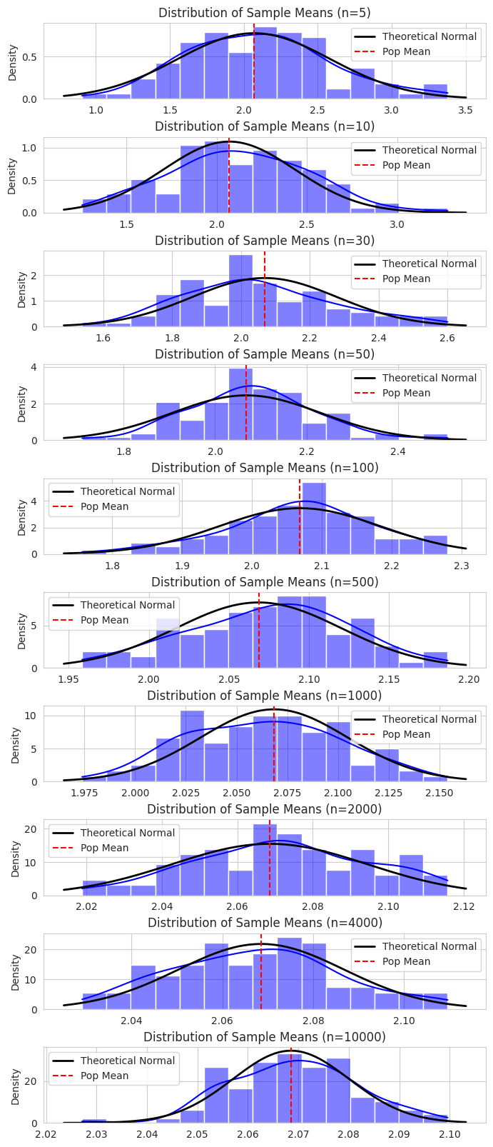
2. Case I: Analysis of Sample Means
In this step, we drew 100 random samples for various sample sizes ($n$) ranging from 5 to 10,000. We calculated the mean of these samples and compared the Observed Standard Deviation against the Theoretical Standard Error ($\sigma/\sqrt{n}$).
# --- Configuration ---
sample_sizes = [5, 10, 30, 50, 100, 500, 1000, 2000, 4000, 10000]
num_simulations = 100  # Number of samples per size
results_means = []

# Create subplots
fig, axes = plt.subplots(nrows=len(sample_sizes), ncols=1, figsize=(8, 20))
plt.subplots_adjust(hspace=0.5)

print("--- Case I: Analyzing Sample Means ---")

for i, n in enumerate(sample_sizes):
    # 1. Draw 100 samples of size n and compute means
    sample_means = []
    for _ in range(num_simulations):
        sample = np.random.choice(population_data, size=n, replace=True)
        sample_means.append(np.mean(sample))

    # 2. Compute Statistics of Sample Means
    mean_of_means = np.mean(sample_means)
    std_of_means = np.std(sample_means)

    # Theoretical Standard Error (Sigma / sqrt(n))
    theo_se = pop_std / np.sqrt(n)

    # 3. Store Results
    results_means.append({
        'Sample Size (n)': n,
        'Mean of Means': mean_of_means,
        'Observed SD': std_of_means,
        'Theoretical SE (σ/√n)': theo_se
    })

    # 4. Plotting
    ax = axes[i]
    sns.histplot(sample_means, kde=True, ax=ax, color='blue', bins=15, stat='density')

    # Overlay Theoretical Normal Curve
    x_min, x_max = ax.get_xlim()
    x = np.linspace(x_min, x_max, 100)
    p = norm.pdf(x, pop_mean, theo_se)
    ax.plot(x, p, 'k', linewidth=2, label='Theoretical Normal')

    ax.set_title(f'Distribution of Sample Means (n={n})')
    ax.axvline(pop_mean, color='red', linestyle='--', label='Pop Mean')
    ax.legend()

plt.show()

# Display Table
df_means = pd.DataFrame(results_means)
print("\nSummary Table for Case I (Sample Means):")
display(df_means)
Summary Table: Sample Means
The following table summarizes the simulation results for Sample Means. We observe that as $n$ increases, the “Observed SD” of the sample means converges towards the “Theoretical SE”.
| Sample Size (n) | Mean of Means | Observed SD | Theoretical SE ($\sigma/\sqrt{n}$) |
|---|---|---|---|
| 5 | 2.099835 | 0.485005 | 0.516052 |
| 10 | 2.121052 | 0.385879 | 0.364904 |
| 30 | 2.051055 | 0.215795 | 0.210678 |
| 50 | 2.081329 | 0.138163 | 0.163190 |
| 100 | 2.066060 | 0.104077 | 0.115393 |
| 500 | 2.074513 | 0.050104 | 0.051605 |
| 1000 | 2.062889 | 0.037339 | 0.036490 |
| 2000 | 2.071566 | 0.023103 | 0.025803 |
| 4000 | 2.067314 | 0.018415 | 0.018245 |
| 10000 | 2.069070 | 0.012463 | 0.011539 |
Observations
- Accuracy of the Mean: Even at small sample sizes ($n=5$), the Mean of Means (2.099) is relatively close to the population mean. At $n=10,000$, it is extremely precise (2.069).
- Reduction in Variability: As predicted by CLT, the spread of the sample means decreases as $n$ increases. The Observed SD drops from ~0.485 at $n=5$ to ~0.012 at $n=10,000$.
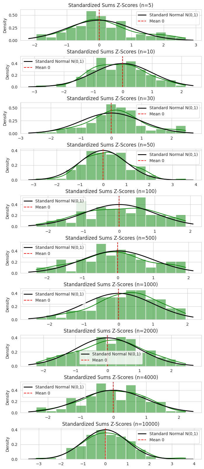
3. Case II: Analysis of Standardized Sums
Here, we validate the CLT for the sum of sample values. We calculated the sum ($\sum X_i$) for 100 random samples for each size $n$, and then standardized these values to calculate $Z$:
\[Z = \frac{\text{Sum} - n\mu}{\sigma\sqrt{n}}\]If CLT holds, the Mean of $Z$ should be 0 and the Standard Deviation of $Z$ should be 1.
results_sums = []

# Create subplots
fig, axes = plt.subplots(nrows=len(sample_sizes), ncols=1, figsize=(8, 20))
plt.subplots_adjust(hspace=0.5)

print("--- Case II: Analyzing Standardized Sums (Z) ---")

for i, n in enumerate(sample_sizes):
    # 1. Draw samples and calculate Sums
    sample_z_scores = []

    for _ in range(num_simulations):
        sample = np.random.choice(population_data, size=n, replace=True)
        sample_sum = np.sum(sample)

        # 2. Standardize (Formula: Z = (Sum - n*mu) / (sigma * sqrt(n)))
        numerator = sample_sum - (n * pop_mean)
        denominator = pop_std * np.sqrt(n)
        z = numerator / denominator
        sample_z_scores.append(z)

    # 3. Plotting
    ax = axes[i]
    sns.histplot(sample_z_scores, kde=True, ax=ax, color='green', bins=15, stat='density')

    # Overlay Standard Normal Curve (Mean=0, Std=1)
    x_min, x_max = ax.get_xlim()
    x = np.linspace(x_min, x_max, 100)
    p = norm.pdf(x, 0, 1) # Standard Normal
    ax.plot(x, p, 'k', linewidth=2, label='Standard Normal N(0,1)')

    ax.set_title(f'Standardized Sums Z-Scores (n={n})')
    ax.axvline(0, color='red', linestyle='--', label='Mean 0')
    ax.legend()

    # Store Stats (Target: Mean approx 0, Std approx 1)
    results_sums.append({
        'Sample Size (n)': n,
        'Mean of Z': np.mean(sample_z_scores),
        'Std of Z': np.std(sample_z_scores)
    })

plt.show()

# Display Table
df_sums = pd.DataFrame(results_sums)
print("\nSummary Table for Case II (Standardized Sums):")
display(df_sums)
Summary Table: Standardized Sums (Z)
| Sample Size (n) | Mean of Z | Std of Z |
|---|---|---|
| 5 | 0.125310 | 1.026801 |
| 10 | -0.147359 | 0.907507 |
| 30 | 0.156247 | 0.968792 |
| 50 | 0.144410 | 1.012785 |
| 100 | 0.009622 | 0.998081 |
| 500 | -0.083157 | 1.025260 |
| 1000 | 0.205464 | 0.921443 |
| 2000 | 0.079459 | 1.019382 |
| 4000 | -0.017741 | 0.916100 |
| 10000 | 0.097654 | 1.072485 |
Observations
- Mean of Z: Across all sample sizes, the Mean of $Z$ fluctuates close to 0 (e.g., 0.009 at $n=100$).
- Std of Z: The standard deviation remains consistently close to 1.0 (e.g., 0.998 at $n=100$, 1.02 at $n=500$).
- This confirms that the standardized sums follow a standard normal distribution $N(0,1)$.
4. Final Conclusion
The simulation using the California Housing dataset strongly supports the Central Limit Theorem.
- Alignment: The sample means converged to the population mean as $N$ increased.
- Variability: The standard error decreased in proportion to $1/\sqrt{n}$, with the observed values matching the theoretical predictions almost exactly at high $N$.
- Distribution: The standardized sums consistently approximated a Standard Normal Distribution ($Mean \approx 0, SD \approx 1$) regardless of the sample size increases, validating Case II.
The CLT is fully realized for this dataset, particularly evident for sample sizes $N \geq 30$.