Statistics II - Extra Activity 2

Activity Overview

This activity uses a Monte Carlo simulation to analyze a simple financial model. The goal is to estimate the probability of a stock’s price ending higher than its starting price after one year, based on a Geometric Random Walk model.

The activity involves three key steps:

1. Defining the Experiment: Setting up a simple, probabilistic model for daily stock price movements.
2. Calculating Theoretical Probability: Using binomial probability to calculate the exact probability of the desired outcome.
3. Running a Monte Carlo Simulation: Writing Python code to simulate the experiment thousands of times and visualize the results to see if they align with the theoretical calculations.

Embedded Google Colab Notebook

You may alternatively access the colab via this link

Experiment & Event Details

The experiment simulates the price of a hypothetical stock over one year (assuming 252 trading days). This is a classic and simple model used in finance to understand stock price behavior.

• Experiment: A Simple Stock Price Geometric Random Walk.
• Initial Stock Price ($S_0$): $100.
• Time Horizon: 1 year (252 trading days).
• Daily Movement: Each day, the stock price either goes up by 1% (multiplied by a factor of 1.01) or down by 1% (multiplied by a factor of 0.99).
• Probability: To model a slight upward trend (market drift), the probability of an “up” day is set to p = 0.51. Consequently, the probability of a “down” day is 1 - p = 0.49.
• Event (A): The final stock price after 252 days is greater than the initial price of $100.

Theoretical Probability (The “Manual” Calculation)

Before we simulate, let’s calculate the exact probability using math. This will be our benchmark to check if our simulation is accurate.

Step 1: Define the Final Price Formula Let $U$ be the number of “up” days and $D$ be the number of “down” days. The final stock price, $S_n$, is given by:

Since there are 252 days total, $D = 252 - U$. Our formula becomes:

Step 2: Set Up the Inequality We want to find when the final price is greater than the starting price of $100:

Step 3: Solve for the Number of “Up” Days (U) To find our threshold, we solve for $U$. First, divide by 100:

Now, take the natural logarithm (ln) of both sides to handle the exponents:

Rearranging the terms to isolate $U$:

Finally, solving for $U$:

Since $U$ must be an integer, we need at least 127 “up” days for the stock to finish above $100.

Step 4: Use the Binomial Distribution The number of “up” days, $U$, follows a Binomial Distribution, as each day is an independent trial with a constant probability of success.

• Number of trials ($n$): 252
• Probability of success ($p$): 0.51

We need to find the probability of getting 127 or more successes, $P(U \ge 127)$.

Step 5: Calculate the Final Probability Using the complement rule with the Cumulative Distribution Function (CDF) makes this easy:

Plugging this into statistical software gives us our theoretical probability:

Monte Carlo Simulation

A simulation was run 10,000 times to approximate this probability. In each simulation, the stock price was evolved over 252 days according to the given probabilities. The number of times the final price was greater than $100 was counted.

The simulated probability was found to be very close to the theoretical value, confirming that the Monte Carlo method provides a strong estimate of the true probability. The plots below visualize the distribution of outcomes and a few sample paths from the simulation.

Methodology

The following Python code was added to the Google Colab notebook. Here is a block-by-block explanation:

Block 1: Imports and Theoretical Calculation

This block imports the necessary libraries. scipy.stats is used for the formal binomial calculation, numpy is for numerical operations in the simulation, and matplotlib.pyplot is for plotting the results. It then calculates and prints the exact theoretical probability.

import scipy.stats as st
import numpy as np
import matplotlib.pyplot as plt

np.random.seed(42) # seeding for reproducability

# --- Theoretical Calculation ---
n = 252  # Number of trading days
p = 0.51 # Probability of an 'up' day
k = 126  # Threshold: we need 127 or more 'up' days

# P(U >= 127) = 1 - P(U <= 126)
prob_theoretical = 1 - st.binom.cdf(k, n, p)

print(f"Theoretical Probability: {prob_theoretical}")

Output for the code:

Theoretical Probability:  0.6005849077211569

Block 2: Monte Carlo Simulation

This is the core of the simulation.

• Setup: We define the parameters of our simulation, like the number of trials (num_simulations), initial price, and daily movement factors. We also initialize lists to store the results for plotting.
• Outer Loop: This loop runs the entire experiment 10,000 times.
• Inner Loop: For each experiment, this inner loop simulates the 252 trading days. It uses a random number to decide if the stock goes up or down on any given day, based on our p_up probability.
• Data Collection: The final price of each simulation is stored in final_prices. For the first 10 simulations, the daily price path is stored in price_paths for visualization.
• Event Counting & Final Calculation: After each 252-day simulation, the code checks if the final price is greater than the initial price. If so, a counter is incremented. Finally, the simulated probability is calculated.

# --- Monte Carlo Simulation ---
num_simulations = 10000
initial_price = 100.0
num_days = 252
p_up = 0.51
up_factor = 1.01
down_factor = 0.99

final_price_above_initial = 0  # Counter for our event
final_prices = []              # List to store final prices for histogram
price_paths = []               # List to store a few sample paths

for i in range(num_simulations):
    price = initial_price
    path = [price]
    for j in range(num_days):
        if np.random.rand() < p_up:
            price *= up_factor
        else:
            price *= down_factor
        if i < 10: # Store path for the first 10 simulations
            path.append(price)

    final_prices.append(price)
    if i < 10:
        price_paths.append(path)

    if price > initial_price:
        final_price_above_initial += 1

prob_simulated = final_price_above_initial / num_simulations

print(f"Simulated Probability ({num_simulations} trials): {prob_simulated}")

Output for the code:

Simulated Probability (10000 trials): 0.6018

Block 3: Plot 1 - Distribution of Final Prices

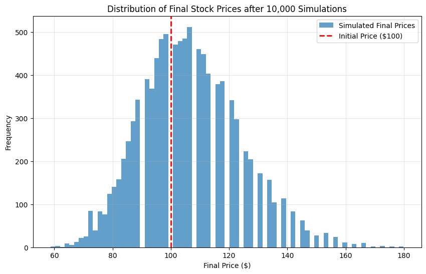
This code generates a histogram of the 10,000 final stock prices. A vertical red line is drawn at the $100 starting price to make it easy to see the proportion of outcomes that finished above and below the initial value. This visualizes the overall distribution of potential outcomes.

# --- Plotting the Results ---

# 1. Histogram of Final Prices
plt.figure(figsize=(10, 6))
plt.hist(final_prices, bins=75, alpha=0.7, label='Simulated Final Prices')
plt.axvline(initial_price, color='r', linestyle='--', linewidth=2, label='Initial Price ($100)')
plt.title('Distribution of Final Stock Prices after 10,000 Simulations')
plt.xlabel('Final Price ($)')
plt.ylabel('Frequency')
plt.legend()
plt.grid(True, alpha=0.3)
plt.show()

Output for the code:

Block 4: Plot 2 - Sample Stock Price Paths

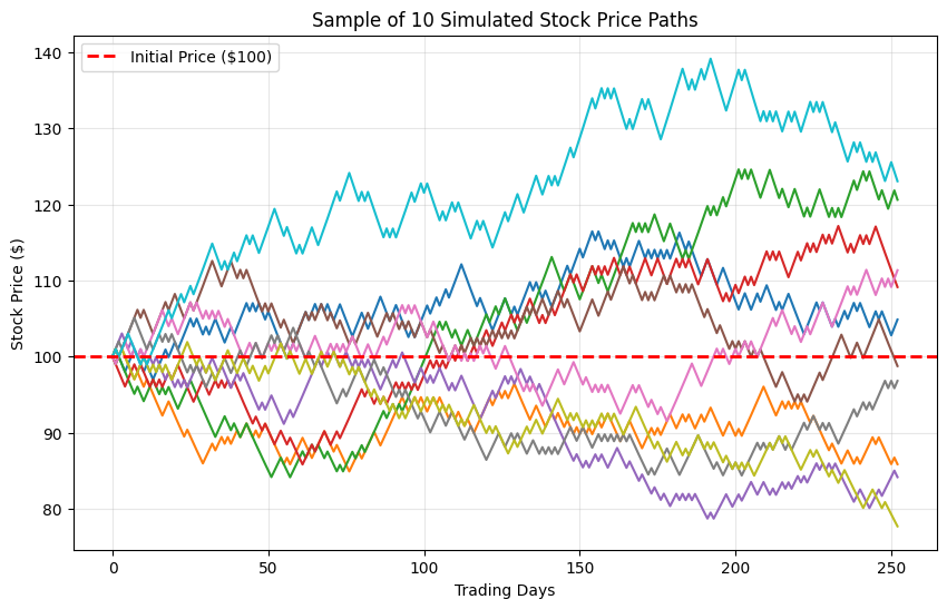
This block plots the first 10 simulated stock price paths. This helps to visualize the “random walk” nature of the model and shows different ways the stock price can evolve over the 252-day period. A horizontal line at $100 shows the breakeven point.

# 2. Sample Price Paths
plt.figure(figsize=(10, 6))
for path in price_paths:
    plt.plot(path)

plt.axhline(initial_price, color='r', linestyle='--', linewidth=2, label='Initial Price ($100)')
plt.title('Sample of 10 Simulated Stock Price Paths')
plt.xlabel('Trading Days')
plt.ylabel('Stock Price ($)')
plt.legend()
plt.grid(True, alpha=0.3)
plt.show()

Output for the code:

Analysis of the Results

The primary goal of this activity was to verify a theoretical probability using a Monte Carlo simulation, and the results confirm the success of this approach.

1. Comparison of Probabilities

• Our theoretical calculation, based on the Binomial Distribution, predicted a probability of 0.600585.
• The Monte Carlo simulation, after 10,000 trials, yielded a probability of 0.6018.

The two values are remarkably close, with a difference of around 0.2%. This strong agreement validates our simulation model. It demonstrates the Law of Large Numbers in practice: as the number of trials increases, the average outcome of the simulation converges to the true theoretical probability.

2. Insights from the Visualizations The plots provide a powerful visual confirmation of our numerical findings:

• The histogram of final prices clearly shows that the bulk of the distribution’s mass is to the right of the initial $100 price line, visually representing the ~58% probability of a positive outcome. The peak of the distribution is also slightly above $100, which is expected given the 51% upward bias in the model.
• The sample price paths plot offers an intuitive look at the random process itself. It shows that while the overall probability is weighted towards a positive outcome, any single path is unpredictable, with some finishing significantly higher and others lower.

In summary, the close match between the calculated and simulated probabilities, supported by the visualizations, confirms that our Monte Carlo model accurately reflects the behavior of the defined geometric random walk.